
159 lines
8.9 KiB
Markdown
159 lines
8.9 KiB
Markdown
# SLO formulas implementation in PromQL step by step
|
||
|
||
- **期号**: SRE Weekly Issue #419(2024-04-07)
|
||
- **作者**: Michał Kaźmierczak
|
||
- **链接**: https://mkaz.me/blog/2024/slo-formulas-implementation-in-promql-step-by-step/
|
||
|
||
## 简介
|
||
|
||
> I want to present real-life examples of both availability and latency SLOs, as they are more nuanced than they may initially appear. Also, I find it worthwhile sharing a detailed guide as it showcases uncommon uses of PromQL and demonstrates the language’s versatility.
|
||
|
||
## 正文
|
||
|
||
# SLO formulas implementation in PromQL step by step
|
||
|
||
## Theory
|
||
|
||
In engineering, perfection isn’t optimal. Even though a service that is continuously up and always responds with the expected latency<sup>[\[1\]](https://mkaz.me#footnotes)</sup> might sound desirable, it would require too expensive resources and overly conservative practices. To maintain the expectations and prioritize engineering resources, it’s common to define and publish **Service Level Objectives (SLO)**.
|
||
|
||
An **SLO defines the tolerable ratio of measurements meeting the target value to all measurements recorded within a specified time interval.**
|
||
|
||
To break it down, I believe that a properly formulated **SLO** consists of four segments:
|
||
|
||
1. Definition of the metric (what’s being measured).
|
||
2. Target value.
|
||
3. Anticipated ratio of good (meeting the target) to all measurements, typically expressed in percentages.
|
||
4. Time interval over which the SLO is considered.
|
||
|
||
A simple **availability SLO** could be:
|
||
|
||
- `a service is up 99.99% of the time over a week period` - the metric is *the service availability* (implicit)
|
||
- the target value is that it’s *up*
|
||
- the anticipated good to all ratio is *99.99%*
|
||
- the considered time interval is *week*
|
||
- the metric is
|
||
|
||
An example of **latency SLO** could be:
|
||
|
||
- `the latency of 99% of requests is less than or equal 250ms over a week period` - the metric is the *requests latency*
|
||
- the target value is *less than or equal 250ms*
|
||
- the anticipated good to all ratio is *99%*
|
||
- the considered time interval is *week*
|
||
- the metric is the
|
||
|
||
Having an SLO defined, a service operator needs to deliver a calculation that tells the reality. The remainder of this article is a step by step guide on how to implement availability and latency SLO formulas with the Prometheus monitoring system.
|
||
|
||
## Practice - SLO formulas with PromQL step by step
|
||
|
||
There are plenty of resources out there about SLO calculation. Moreover, there are off-the-shelf solutions for getting SLOs from metrics<sup>[\[2\]](https://mkaz.me#footnotes)</sup>.
|
||
|
||
OK then, why add one more resource on the topic? I want to present real-life examples of both availability and latency SLOs, as they are more nuanced than they may initially appear. Also, I find it worthwhile sharing a detailed guide as it showcases uncommon uses of PromQL and demonstrates the language’s versatility.
|
||
|
||
### Formula for availability SLO
|
||
|
||
Let’s look again at our SLO:
|
||
|
||
```
|
||
A service is up 99.99% of the time over a week period.
|
||
```
|
||
To reason about a service’s availability we need a metric that indicates whether a service is up or down. Additionally, we need to sample this metric at regular time intervals. This allows us to divide the count of samples when the service reported as up by the count of all time intervals in the observed period. This gives us our SLO.
|
||
|
||
Prometheus delivers the `up` metric (quite an accurate naming) for every scrape target. It’s a gauge which reports `1` when the scrape succeeded and `0` if the scrape failed. Given its simplicity, it’s a very good proxy of the service’s availability (however, it’s still prone to false negatives and false positives).
|
||
|
||
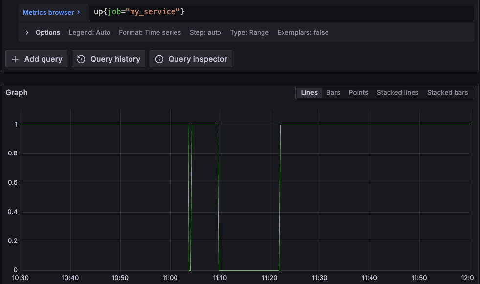
Let’s consider the following plot of an `up` metric:
|
||
|
||
|
||
|
||
|
||
This service was sampled every 15s. The time range is from 10:30:00 to 12:00:00 (1h30m inclusive - 361 samples). We can observe two periods when the service was down: `from 11:03:45 to 11:04:00` and `from 11:09:45 to 11:21:45`. This gives us `2 + 49 = 51` samples missing the target and `361 - 51 = 310` samples meeting the target.
|
||
|
||
Therefore the SLO is `(310 / 361) * 100 = 85.87%`. How to get this number with PromQL? Intuitively, we could count good samples and all samples (with `count_over_time`), and then calculate the ratio. However, given that the `up` metric is a gauge reporting either `0` or `1` we can do a trick and use the `avg_over_time` function:
|
||
|
||
```
|
||
avg_over_time(
|
||
up{job="my_service"}[90m:]
|
||
) * 100
|
||
=> 85.87257617728531
|
||
```
|
||
For production readiness, I recommend using [instant query](https://prometheus.io/docs/prometheus/latest/querying/api/#instant-queries) and adjust the range. Also, see the footnotes if you suffer from periodic metric absence<sup>[\[3\]](https://mkaz.me#footnotes)</sup>.
|
||
|
||
### Formula for latency SLO
|
||
|
||
Let’s recity our latency SLO:
|
||
|
||
```
|
||
The latency of 99% of requests is less than or equal 250ms over a week period.
|
||
```
|
||
For an accurate calculation, we need the count of requests that took less than or 250ms and the count of all requests. It turns out that it is a rare luxury, though. It actually means that you either have:
|
||
|
||
- the service instrumented upfront with a counter that increments when a request takes less than or 250ms, along with another counter that increments for every request;
|
||
- a histogram metric with one of the buckets set to `0.25` , which is the same as the first point as a histogram is essentially a set of counters.
|
||
|
||
Assuming you have the histogram metric with the `0.25` bucket, the query is:
|
||
|
||
```
|
||
sum(
|
||
increase(http_request_latency_seconds_bucket{job="my_service",le="0.25"}[7d])
|
||
) * 100 /
|
||
sum(
|
||
increase(http_request_latency_seconds_bucket{job="my_service",le="+Inf"}[7d])
|
||
)
|
||
=> 99.958703283089
|
||
```
|
||
Ok, but what to do when such counters aren’t available?
|
||
|
||
### Formula for latency SLO with percentiles
|
||
|
||
Another approach to latency SLOs is setting expectations regarding percentiles, which is a common real-life example. It gives the flexibility in testing different target values without the need of re-instrumentation. However, I suggest to refrain from relying solely on percentiles in SLOs for several reasons:
|
||
|
||
- it’s an aggregate view, so it may hide certain characteristics of the service; a ratio of two counters offers way more straightforward understanding;
|
||
- combining percentiles from different services can be tricky; for example, averaging percentiles is possible only for services having the same latency distribution (almost impossible) or by calculating a weighted average (also almost impossible);
|
||
- the SLO gets more complicated, making it difficult to reason about — especially for non-SRE people who are also users of the SLO.
|
||
|
||
Nonetheless, an example of such an SLO is:
|
||
|
||
```
|
||
99th percentile of requests latency is lower than 400ms 99% of the time over a week period.
|
||
```
|
||
It can be implemented in PromQL in three steps:
|
||
|
||
1. Calculate the quantile: ```
|
||
histogram_quantile(
|
||
0.99,
|
||
sum by (le) (rate(http_server_request_duration_seconds_bucket[1m]))
|
||
)
|
||
```
|
||

|
||
2. Perform a binary quantization to get a vector of `1` and`0` values corresponding to when the target value is met and not met. It’s a perfect input for our`avg_over_time` function. This is achieved with the`bool` modifier (`<bool 0.4` ).```
|
||
histogram_quantile(
|
||
0.99,
|
||
sum by (le) (rate(http_server_request_duration_seconds_bucket[1m]))
|
||
) <bool 0.4
|
||
```
|
||

|
||
3. Calculate the percentage: ```
|
||
avg_over_time(
|
||
(histogram_quantile(
|
||
0.99,
|
||
sum by (le) (rate(http_server_request_duration_seconds_bucket[1m]))
|
||
) <bool 0.4)[7d:]
|
||
) * 100
|
||
=> 96.66666666666661
|
||
```
|
||
|
||
When you finish prototyping with any of the above formulas, it’s a good practice to define a recording rule for the main metric for an efficient evaluation.
|
||
|
||
## Footnotes
|
||
|
||
1. In this article, ‘latency’ refers to the time it takes for the service to generate a response. I want to clarify it because in some resources it’s used as the time that a request is waiting to be handled.
|
||
2. On this note, I highly recommend getting familiar with [Pyrra](https://github.com/pyrra-dev/pyrra/) .
|
||
3. It’s a common issue that the DB misses certain samples when the monitoring is hosted on the same server as the service having problems. While rethinking the architecture would be ideal, a quick workaround is to reduce all labels from the `up` metric and*fill the gap* with the scalar`vector(0)` . Beware, the consequence is that the absence of the metric is seen as the service being down.```
|
||
avg_over_time(
|
||
(sum(up{job="my_service"}) or vector(0))[90m:]
|
||
) * 100
|
||
```
|
||
|
||
#### Get in touch
|
||
|
||
If for whatever reason you consider it worthwhile to start a conversation with me, please check out the [about](https://mkaz.me/) page to find the available means of communication.
|